Prediction Of Shrinkage Using Neural Networks and Equations Of State
Feb 8, 2021
Authors: Preston Blackburn and Ben Bagby
Equations of state (EOS) are central in making predictions for petroleum allocations. However, commonly used EOS, such as volume translated Peng-Robinson EOS (VTPR-EOS), still deviate from lab results. To improve accuracy many EOS’s continue to add more complexity or tune parameters to better capture the thermodynamics properties of hydrocarbon mixtures.
In this post I go over a way to improve the EOS for shrinkage calculations using a feed forward artificial neural network. Accuracy of the model along with the associated uncertainty will also be analyzed.
Shrinkage is an essential property for allocations of petroleum that describes a change in volume of petroleum liquid after the petroleum goes through a separator with a reduced pressure or raised temperature. Small differences in predicted shrinkage values can lead hundreds of barrels of oil being un-counted.
In this post we overview how a VTPR EOS combined with a neural network can improve the prediction of shrinkage values if at all versus a standalone neural network. In other works, Ahmadi (2015) has shown that artificial neural networks (ANN) using particle swarm optimization (PSO) can be used to accurately estimate bubble point pressure but did not analyze the effect of adding EOS data to the model.
Equations of State Background
Equations of state attempt to accurately predict Pressure, Volume, and Temperature (PVT) behavior of a component or mixture. While many equations of state exist, predicting phase equilibrium properties in petroleum is primarily done with Cubic EOS based on modifications of the van der Waals EOS.
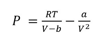
Van der Waals first introduced his EOS which included a and b terms for specific attraction and volume occupied by molecules respectively (Van Der Waals, 1873), shown below.
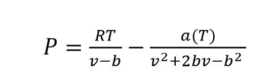
Arguably the most popular EOS to come from the van der Waals EOS was the Peng-Robinson EOS. Peng and Robinson’s EOS modified the alpha function of Soave’s equation by modifying the volume dependency of the attractive term (Peng-Robinson, 1976). This EOS is so effective that it is still used today. However, it is common to add a volume translation when used in practice. The Peng-Robinson EOS is shown below and is the basis for the EOS that was used in this post.
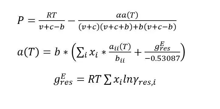
This brings us to the volume translated Peng-Robinson equation with Gibbs free energy mixture parameters. The volume translation adds a component-dependent molar volume correction factor. This correction factor is essential to providing accurate results like shrinkage, since shrinkage is entirely based on liquid volume (Tsai and Chen, 1998). The EOS used in this paper is outlined by the equations below.
Brief Data and Model Overview
The majority of the oil samples are condensates or heavier. The API gravity of the samples ranged from 147.15 to 43.47 with a 25th percentile of 70.18. Shrinkage values ranged from 0.0878 to 0.9947. The 25th percentile of the shrinkage values was 0.8315.
The initial input for this model were pressure, temperature, liquid volume percent (LV%) nitrogen, carbon dioxide, methane, ethane, propane, isobutane, n-butane, isopentane, n-pentane, hexanes (grouped), heptanes plus (C7+), C7+ specific gravity, and C7+ molecular weight.
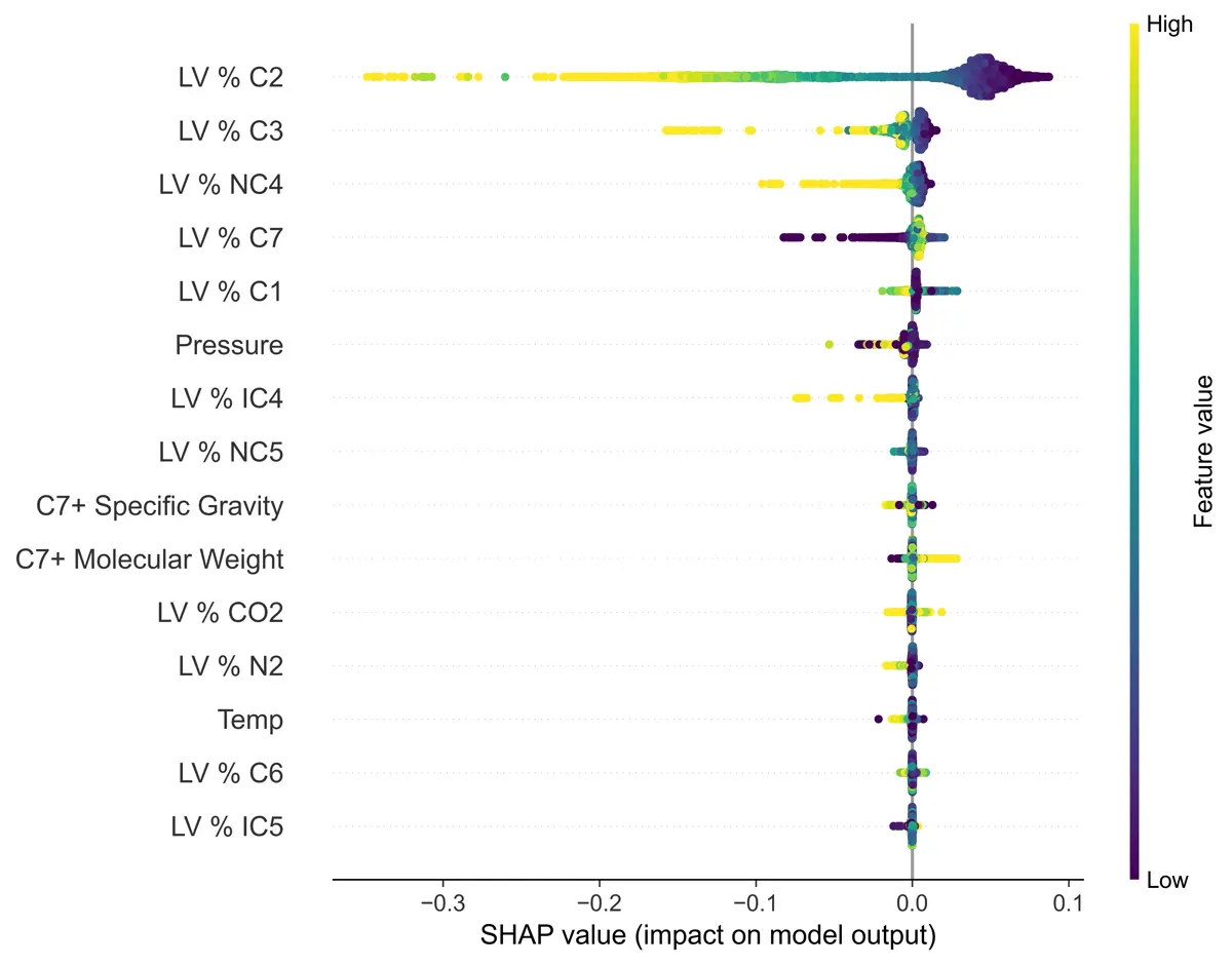
For the sake of brevity, I will not go into any details from my exploratory data analysis. However, I thought it might be interesting showing the SHAP (Shapley Additive exPlanations) plots from the analysis. The SHAP plots can allow the user to gain insights into what the machine learning models are using to predict shrinkage.
The first plot shows feature importance if XGBoost is used as the regression model. The feature importance makes intuitive sense as ethane (C2) and propane (C3) would almost completely flash off while accounting for a more significant portion of the sample than other light ends such as nitrogen and methane. The heptanes plus (C7) fraction makes up the largest portion of the sample and will not flash much when the sample is brought down to lower pressures.
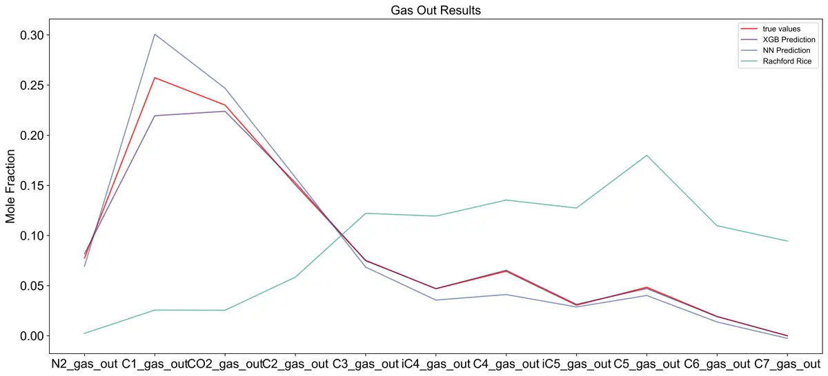
Final Model Results
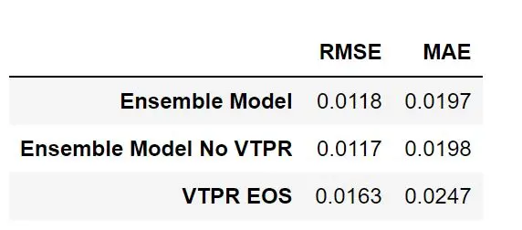
Adding the VTPR EOS results to the model does not seem to significantly impact performance according to the SHAP plot. It is the second least important model out of the 6 models used in the meta model. Results can be seen below.
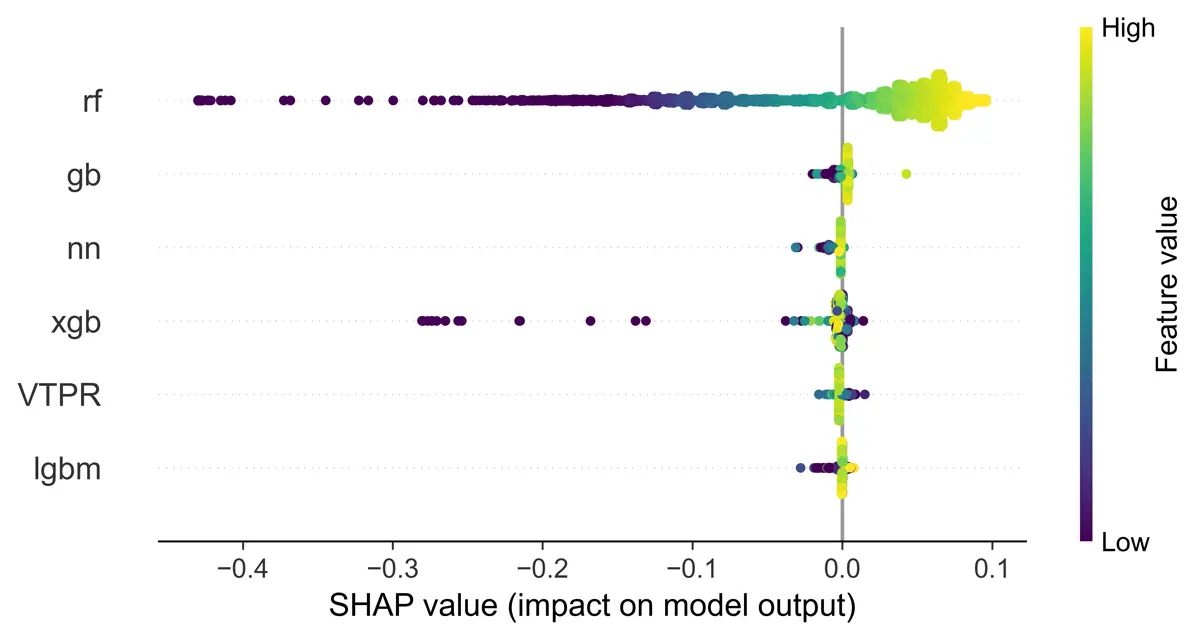
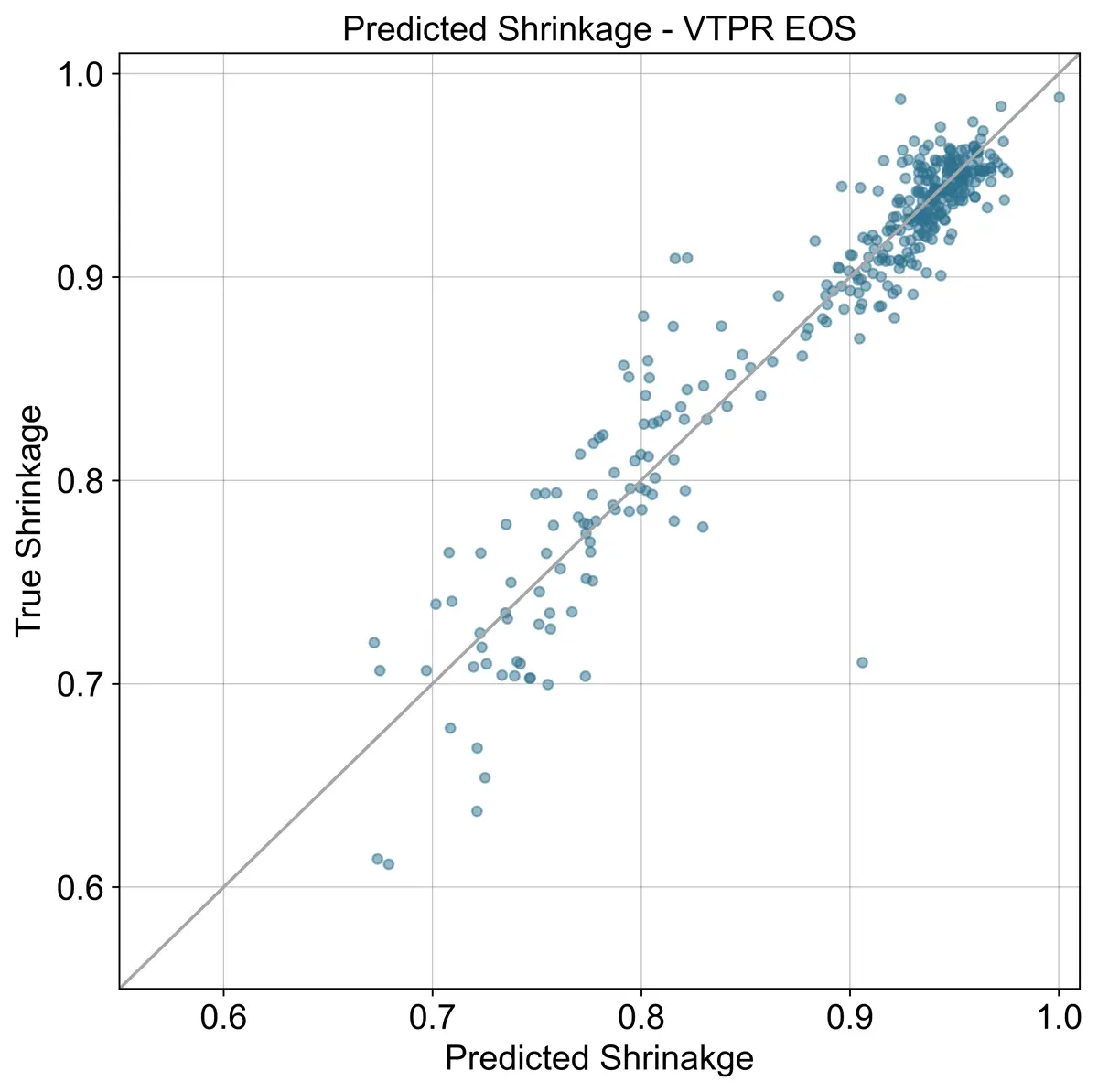
Results confirm this when the models are combined by using a neural network. The VTPR EOS was outperformed by the machine learning model, which was expected based on Ahmadi’s (2015) work.
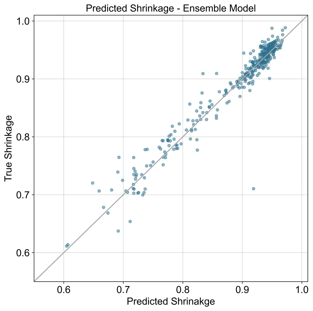
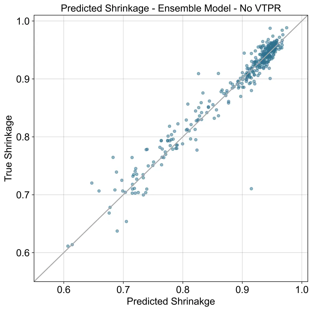
Below three plots are shown comparing the ensemble model with the VTPR EOS results included, without the VTPR EOS, and the results from the VTPR EOS alone. Looking at the summary table, adding the VTPR EOS to the ensemble has almost no impact.
Conclusion
While ML models outperform EOS when sufficient training data is available, EOS will still need to be used when training data is sparse. When flashing to pressures other than ambient much less training data exists, and EOS models will still need to be used.
For this reason, it may be worthwhile to look into using transfer learning to pre-train a neural network with results from an EOS then use lab data to further train the pre-trained model.
To Be Continued in Part 2......
In part two of this post, I will look at using Bayesian methods to produce uncertainty intervals for the shrinkage models. Currently the commonly used EOS models don’t provide any metric of uncertainty despite the known deviation from actual lab data.
In my opinion this has led to the industry overusing EOS results vs physical measurements, as EOS calculations are seen as infallible. By adding uncertainty intervals to my models, I hope to shed more light on the prediction accuracy for various petroleum compositions.
References
-
Abudour, A. M., Mohammad, S. A., Robinson Jr, R. L., & Gasem, K. A. (2013). Volume-translated Peng-Robinson equation of state for liquid densities of diverse binary mixtures. Fluid Phase Equilibria 349: 37-55. doi
-
Ahmadi, M. A., Pournik, M., & Shadizadeh, S. R. (2015). Toward connectionist model for predicting bubble point. Petroleum 307-317. doi
-
Bergstra, J., Yamins, D., Cox, D. D. (2013). Hyperopt: A Python Library for Optimizing the Hyperparameters of Machine Learning Algorithms. Proceedings of the 12th Python in Science Conference. doi
-
Chen, T., and Guestrin, C. (2016). XGBoost: A Scalable Tree Boosting System. Proceedings of the 22nd ACM SIGKDD International Conference. doi
-
Geron, A. (2019). Hands-on Machine Learning with Scikit-Learn and TensorFlow. O'Reilly Media.
-
Hornik, K., Stinchcombe, M., and White, H. (1989). Multilayer Feedforward Networks are Universal Approximators. Neural Networks 2: 359-366. doi
-
Kandula, V. K., Telotte, J. C., & Knopf, F. C. (2013). It's Not as Easy as it Looks: Revisiting Peng–Robinson Equation of State Convergence Issues. International Journal of Mechanical Engineering Education 41(3): 188-202. doi
-
Ke, G., et al. (2017). LightGBM: A Highly Efficient Gradient Boosting Decision Tree. NeurIPS 30. PDF
-
Lundberg, S. M., and Lee, S. I. (2017). A Unified Approach to Interpreting Model Predictions. NeurIPS.
-
Pedregosa, F., et al. (2011). Scikit-learn: Machine Learning in Python. JMLR 12: 2825-2830.
-
Peng, D. Y., & Robinson, D. B. (1976). A new two-constant equation of state. Industrial & Engineering Chemistry Fundamentals 15(1): 59-64. doi
-
Prechelt, L. (1998). Early Stopping – But When? Neural Networks: Tricks of the Trade 55-69. doi
-
Reed, R. D., and Marks, R. J. (1999). Neural Smithing: Supervised Learning in Feedforward Artificial Neural Networks. MIT Press.
-
Srivastava, N., et al. (2014). Dropout: A Simple Way to Prevent Neural Networks from Overfitting. JMLR 15: 1929-1958. link
-
Valderrama, J. O. (2003). The state of the cubic equations of state. Industrial & Engineering Chemistry Research 42(8): 1603-1618. doi