Oil Production Forecasting

Dec 30, 2020

Production forecasting is used to predict the future performance of an oil or gas well. Typically, these predictions are referred to as decline curves because the production of a well decreases with time. Usually, oil and gas wells decline exponentially. Traditionally Arps curves have been used to predict production by taking advantage of this exponential decline rate. However, predictions can be improved using modern machine learning techniques, such as Bayesian deep learning. Bayesian models consider information outside of the dataset, unlike traditional (frequentist) models. Bayesian methods have the advantage of providing uncertainty intervals for the model’s predictions, which frequentist methods typically struggle to produce. Having uncertainty intervals can be useful when evaluating a forecasting model, especially when poor forecasts can be costly.

Below I predict the production rates and associated error of a case study to get experience using Bayesian deep learning techniques. To get a sense of how well the model performs, I compare the results to two other Bayesian models: a Bayesian Arps curve and Facebook’s forecasting model, “Prophet.”

If you would like to know more go to this repo: Programming and Bayesian Methods

Production Data

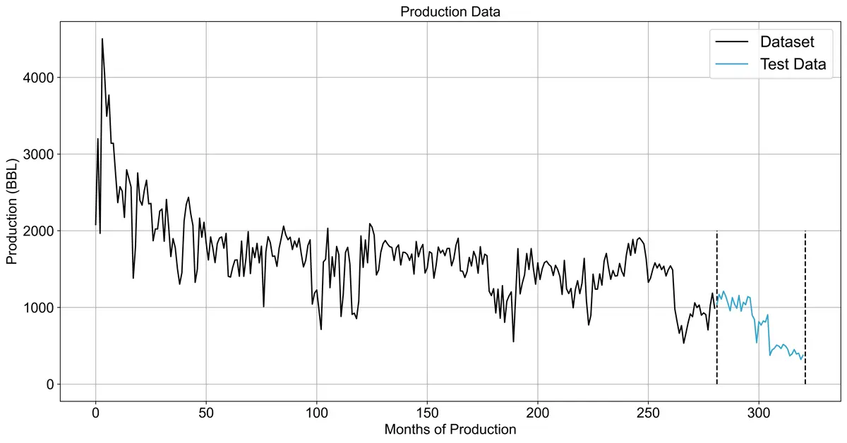
For this case study, data was taken from the Texas Railroad Commission (RRC). This well was chosen because of its long history and typical decline profile. The data was split into two datasets: training (the first 280 months) and test (the remaining 40 months). The models will make predictions on the test dataset, shown by the blue line below.

The dataset can be found on my GitHub: Production Data

Bayesian Neural Network using Monte Carlo Dropout

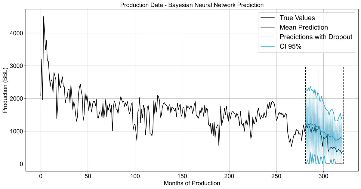
My Bayesian deep learning model’s architecture takes aspects of top-performing neural network architectures and combines them with Monte Carlo (MC) Dropout to approximate a Bayesian prediction. The architecture used is a dilated convolutional neural network (CNN) with LSTM cells, which have been shown to perform well in data science competitions like those hosted by Kaggle. Applying MC dropout can estimate what a Bayesian network might look like while keeping computation costs down. The mean prediction, 95% credible interval, and 50 predictions ran with MC dropout are shown in the graph below. For the 50 predictions, the opacity is turned down to make the mean prediction and credible interval easier to see. The model seems like it might be a little under confident about its forecast, but I will make another post going over the reliability diagram in the future.

ARPs using Bayesian Regression

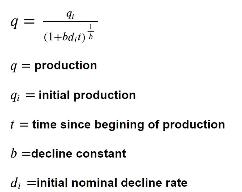
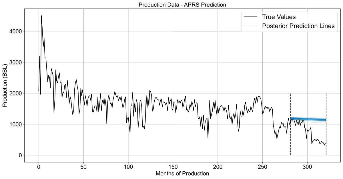
Probabilistic methods can be applied to ARPs curve predictions to simulate various potential predictions. For this model I used the Arps equation mentioned at the beginning of this paper combined with the PyMC3 Python API. For the sake of simplicity, I will not cover specifics such as Markov Chain Monte Carlo (MCMC) methods or Bayesian terminology such as priors and posteriors. 50 of the posterior predictive lines are plotted in the example below.

Arps Equation Used:

Facebook Prophet

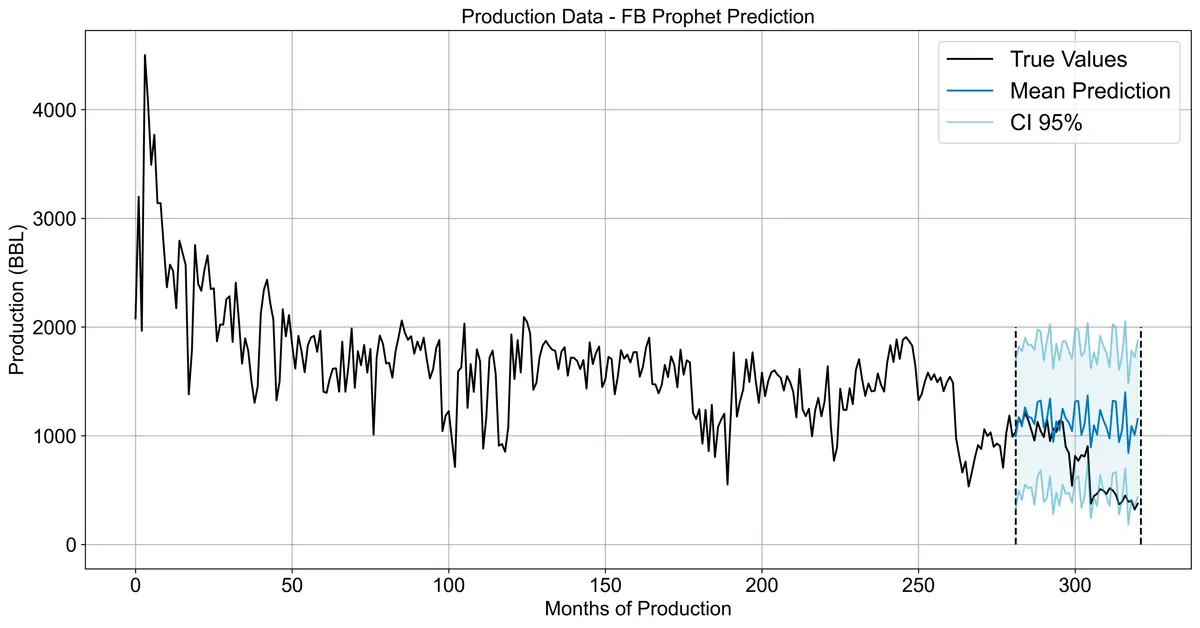
Facebook Prophet uses Bayesian methods for prediction that are easily applied at scale. It is based on a generative additive model that considers changepoints, trends, seasonality, and more. In the model below, the default FB Prophet model was used with minimal tuning. Better results may be obtained by tuning. The uncertainty interval is shown by the light blue lines in the graph below. The model also seems to be overconfident about its uncertainty interval since some of the actual production values are out of range.

Model Comparisons

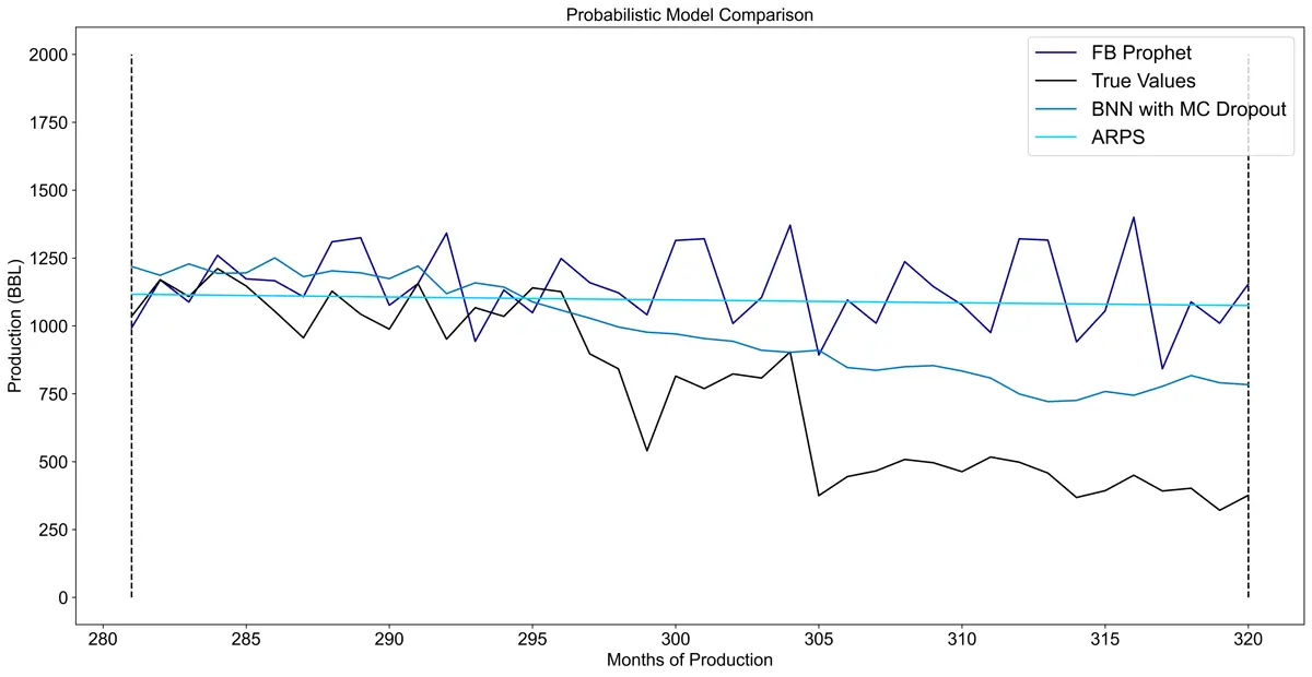
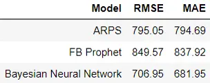
I compare the mean prediction of all three models below for the last 40 months below. As expected, the Bayesian neural network outperforms both the Arps model and Facebook Prophet for this case study. The Bayesian neural network did the best at capturing the drop in production after 295 months. Additional metrics in the performance summary table show that the Bayesian neural network outperforms the other two models for this case study.

Performance Summary:

To Be Continued in Part 2...

The results could potentially be improved even further if additional data were fed into the network, such as the well’s workover history. In a future post, I may investigate adding additional data from the chemical disclosure registry Frac Focus. Furthermore, the model’s performance should be evaluated to see if it is under-confident or overconfident using a reliability diagram.