ML Modeling of Condensate Mixture Properties
Jan 4, 2021
Some liquid analyses in the oil and gas industry can be improved or shortened using machine learning.
One such test is GPA 2013 – an analysis used to determine the composition of oil along with properties such as molecular weight and relative density. Multiple analyses are needed to provide all the necessary information, and this is where machine learning can come in and shorten the process.
We can eliminate an extra analysis that usually takes around 30 minutes by modeling it based on information taken from the other analyses. In fact, 3 out of the 4 analyses of this test can be modeled by a single analysis with only slight losses in accuracy.
In my first model I look at the results with only replacing the 30-minute gas chromatograph (GC) analysis, and in the second I model all the needed results based off only one analysis. By modeling these results, the test time of GPA 2103 can be reduced by 30–60%. Furthermore, this is one of the most common tests done on condensate and crude oils, which means this model could save companies tens of thousands of hours of test time per year.
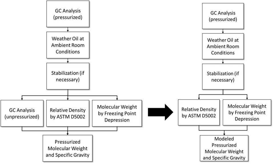
Model Applications
Model 1 Applied to GPA 2103 Process
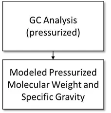
Model 2 Applied to GPA 2103 Process
Since I am modeling the values, I am not limited by what is possible with current laboratory equipment. In current GPA 2103 process unpressurized relative density and molecular weight are measured, but the needed values are pressurized relative density and molecular weight. This is also the reason a second GC test is required.
Brief Data and Model Overview
If you are interested in learning more about the data used for this model and the processes I used to explore and validate the dataset, please reach out to me on LinkedIn. For the sake of keeping this post to a reasonable length I will only go through my modeling process and the results.
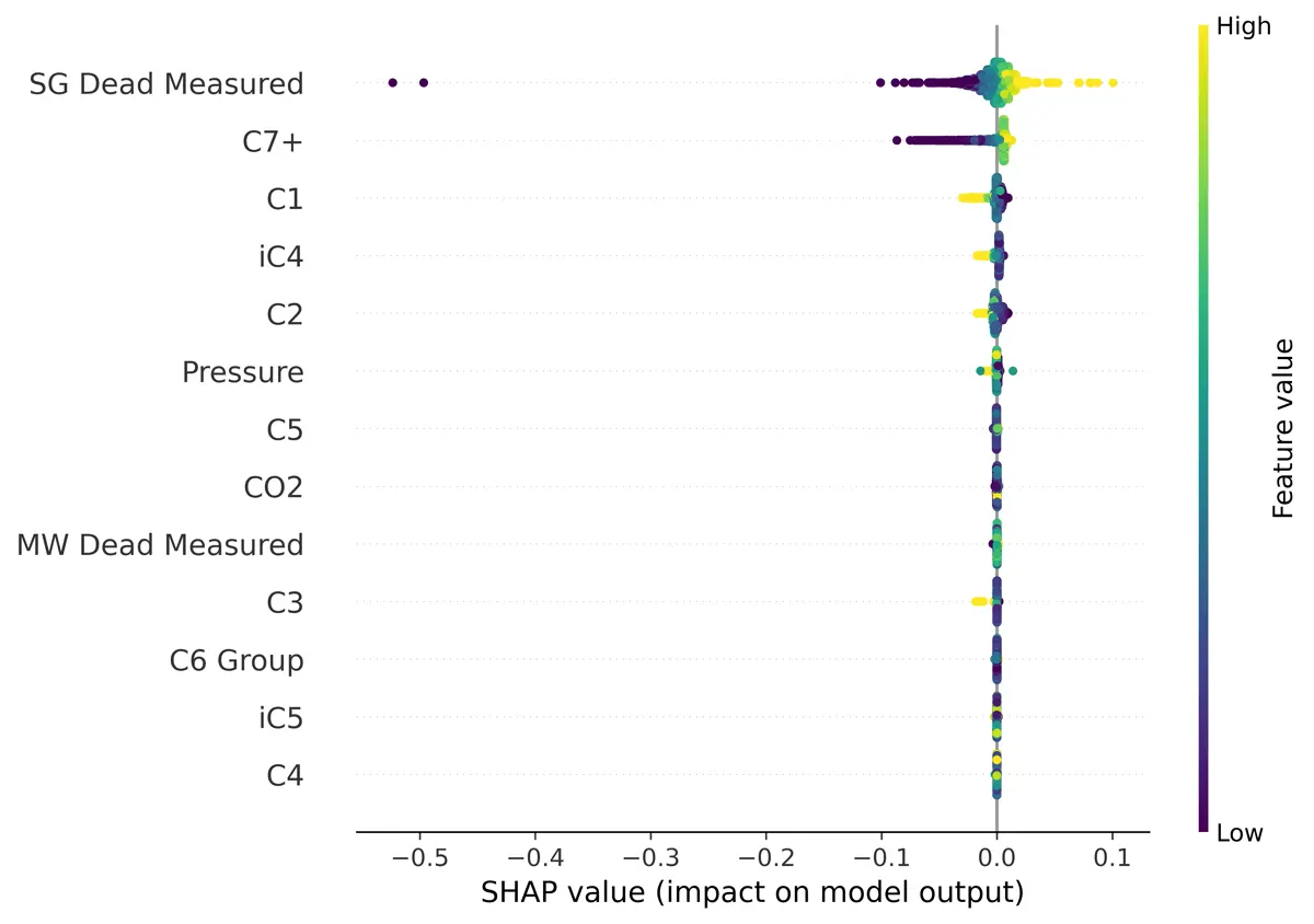
Using SHAP (Shapley Additive exPlanations) I found that the unpressurized molecular weight and relative density were important to modeling the pressurized molecular weight and relative density, as you would expect. That is why I chose to create two models, one without the unpressurized measurements and one including them.
Feature Selection – Molecular Weight
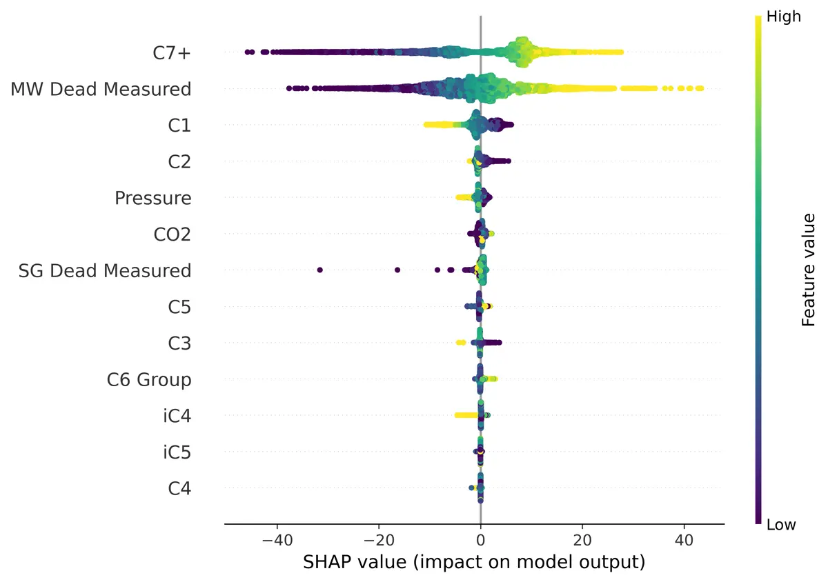 Feature Selection – Relative Density
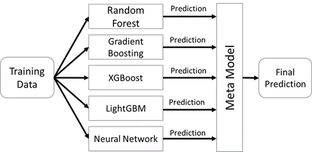
To create the model, I used a stacked ensemble architecture. Linear models, such as linear support vector machines, fit the data poorly, so I left them out of my ensemble. The random forest model and gradient boosting model were taken from Scikit-learn, and the neural networks were created using the Keras API for TensorFlow. I added the XGBoost and LightGBM gradient boosting models because of their well-known high performance.
Ensemble Model Design
Model Results
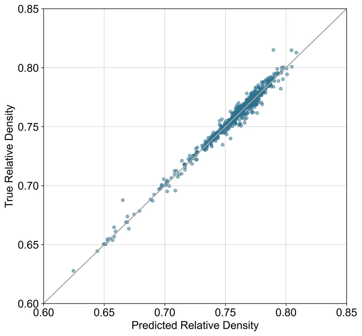
The results of the models for predicting pressurized molecular weight and relative density are shown below. As expected, the models without measured molecular weight and relative density performed slightly worse. However, the decrease in accuracy still might be acceptable given the decreased analysis time.
Modeled Values vs Measured Values
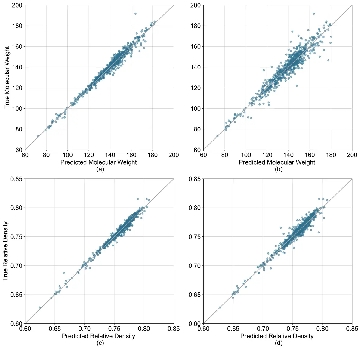
(a) Model 1 molecular weight prediction accuracy. (b) Model 2 molecular weight prediction accuracy.
(c) Model 1 relative density prediction accuracy. (d) Model 2 relative density prediction accuracy.
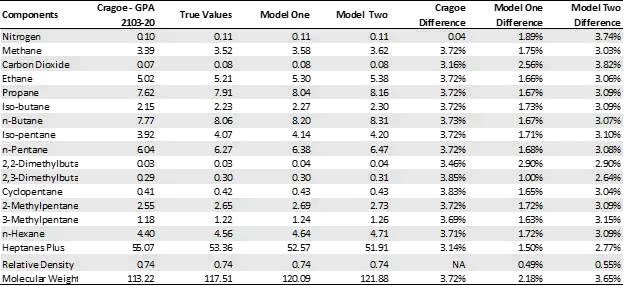
Summary Table
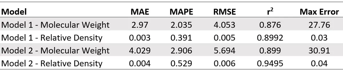
An alternative to measuring molecular weight in GPA 2103 is to use the Cragoe correlation, which predicts unpressurized molecular weight based on measured unpressurized specific gravity.
In the table below the results from the models are compared to GPA 2103 when using the Cragoe correlation for a sample. From those results the models perform similarly, if not better, than using the Cragoe correlation. Furthermore, the time savings are much greater when using the machine learning models compared to the Cragoe correlation.
Case Study Comparison
I was also interested in looking at the uncertainty associated with the models to see if there are any samples that the models should not be applied to. To analyze uncertainty, I used negative logarithmic loss function on the meta model. With the negative log loss function both the mean and variance can be produced using maximum likelihood methods.
Uncertainty vs Predicted Values
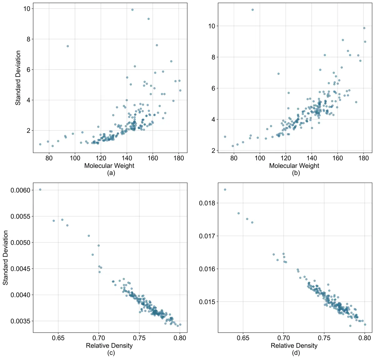 (a) Model 1 molecular weight vs predicted standard deviation.
(b) Model 2 molecular weight vs predicted standard deviation.
(c) Model 1 relative density vs predicted standard deviation.
(d) Model 2 relative density vs predicted standard deviation.
Conclusion
Implementing these models saves a lot of analysis time with minimal accuracy loss. As the oil and gas industry continues to push for increased efficiency, more time-saving measures such as the one described in this post will become necessary.
References
- Bergstra, J., Yamins, D., Cox, D. D. 2013. Hyperopt: A Python Library for Optimizing the Hyperparameters of Machine Learning Algorithms. Proceedings of the 12th Python in Science Conference. Citeseer. doi:http://dx.doi.org/10.1.1.704.3494.
- Bishop, C. M. 1994. Mixture Density Networks. PDF.
- Breiman, L. 1996. Bagging Predictors. Machine Learning (24): 123–140. doi:https://doi.org/10.1023/A:1018054314350.
- Breiman, L. 2001. Random Forests. Machine Learning 45(1): 5–32. doi:http://dx.doi.org/10.1023/a:1010933404324.
- Chen, T., and Guestrin, C. 2016. XGBoost: A Scalable Tree Boosting System. In Proceedings of the 22nd ACM SIGKDD International Conference on Knowledge Discovery and Data Mining. New York, NY. 785–794. doi:https://doi.org/10.1145/2939672.2939785.
- Cragoe, C. S. 1929. Thermodynamic Properties of Petroleum Products. Bureau of Standards, U.S. Dept. of Commerce, Misc. Publications No. 97.
- Friedman, J. H. 2001. Greedy Function Approximation: A Gradient Boosting Machine. Annals of Statistics 1189–1232. doi:http://dx.doi.org/10.1214/aos/1013203451.
- Geron, A. 2019. Hands-On Machine Learning with Scikit-Learn and TensorFlow: Concepts, Tools, and Techniques to Build Intelligent Systems. O’Reilly Media.
- Hornik, K., Stinchcombe, M., and White, H. 1989. Multilayer Feedforward Networks Are Universal Approximators. Neural Networks, Vol 2: 359–366. doi:http://dx.doi.org/10.1016/0893-6080(89)90020-8.
- Ke, G., Meng, Q., Finley, T., Wang, T., Chen, W., Ma, W., Ye, Q., and Liu, T. 2017. LightGBM: A Highly Efficient Gradient Boosting Decision Tree. Advances in Neural Information Processing Systems 30. PDF.
- Kursa, M. B., and Rudnicki W. R. 2010. Feature Selection with the Boruta Package. Statistical Software Vol. 36, Issue 11: 1–13.
- Pedregosa, F., Varoquaux, G., Gramfort, A., Michel, V., Thirion, B., Grisel, O., Blondel, M., Prettenhofer, P., Weiss, R., Dubourg, V., Vanderplas, J., Passos, A., Cournapeau, D., Brucher, M., Perrot, M., and Duchesnay, E. 2011. Scikit-learn: Machine Learning in Python. Journal of Machine Learning Research, Vol 12: 2825–2830.
- Prechelt, L. 1998. Early Stopping – But When? Neural Networks: Tricks of the Trade 55–69. doi:http://dx.doi.org/10.1007/3-540-49430-8_3.
- Srivastava, N., Hinton, G., Krizhevsky, A., Sutskever, I., Salakhutdinov, R. 2014. Dropout: A Simple Way to Prevent Neural Networks from Overfitting. Journal of Machine Learning Research 15: 1929–1958. Link.
- Valderrama, J. O. 2003. The State of the Cubic Equations of State. Industrial & Engineering Chemistry Research 42(8): 1603–1618. doi:https://doi.org/10.1021/ie020447b.